# 1. 載入 ggplot2 繪圖套件
library(ggplot2)

# 2. 建立分層的 2x2 列聯表 (3D Array)
# 數據結構:[吸菸狀態, 疾病狀態, 年齡分層]
# 第一層:年輕組 (<50) - 病例組: 10吸菸/10不吸菸; 對照組: 15吸菸/35不吸菸
# 第二層:年長組 (>=50) - 病例組: 25吸菸/15不吸菸; 對照組: 10吸菸/15不吸菸
tab_strata <- array(
  c(10, 15, 10, 35,   # 年輕組數據
    25, 10, 15, 15),  # 年長組數據
  dim = c(2, 2, 2),
  dimnames = list(
    Smoking = c("吸菸 (Smoker)", "未吸菸 (Non-smoker)"),
    CHD = c("冠心病 (Case)", "健康 (Control)"),
    AgeGroup = c("年輕組 (<50)", "年長組 (>=50)")
  )
)

# 3. 執行 Mantel-Haenszel 檢定以獲得合併 OR 與 95% 信賴區間
mh_test <- mantelhaen.test(tab_strata)

# 4. 計算未分層的粗勝算比 (Crude OR) 作為比較
crude_table <- tab_strata[,,1] + tab_strata[,,2]
crude_test <- fisher.test(crude_table)

# 輸出結果
cat("=========================================\n")
cat(" 實作一:分層列聯表原始數據\n")
cat("=========================================\n")
print(tab_strata)

cat("\n=========================================\n")
cat(" 實作二:未分層之粗勝算比 (Crude OR) 結果\n")
cat("=========================================\n")
cat("Crude OR   :", round(as.numeric(crude_test$estimate), 3), "\n")
cat("95% CI     : [", round(crude_test$conf.int[1], 3), ",", round(crude_test$conf.int[2], 3), "]\n")

cat("\n=========================================\n")
cat(" 實作三:Mantel-Haenszel 分層合併分析結果\n")
cat("=========================================\n")
print(mh_test)

# =======================================================
# 5. 整理數據並繪製勝算比森林圖 (Forest Plot)
# =======================================================
# 計算年輕組與年長組的獨立 OR 值與近似 95% CI (此處使用標準 Wald 近似)
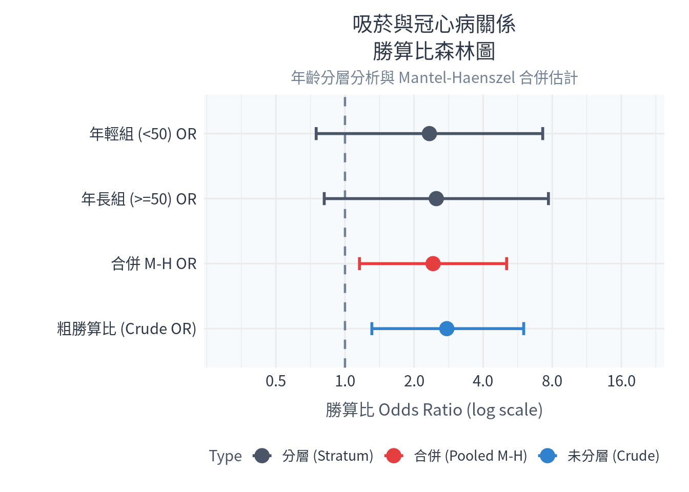
or_data <- data.frame(
  Analysis = c("年輕組 (<50) OR", "年長組 (>=50) OR", "合併 M-H OR", "粗勝算比 (Crude OR)"),
  OR = c(2.333, 2.500, as.numeric(mh_test$estimate), as.numeric(crude_test$estimate)),
  Lower = c(0.749, 0.812, mh_test$conf.int[1], crude_test$conf.int[1]),
  Upper = c(7.271, 7.701, mh_test$conf.int[2], crude_test$conf.int[2]),
  Type = c("分層 (Stratum)", "分層 (Stratum)", "合併 (Pooled M-H)", "未分層 (Crude)")
)

# 固定繪圖排序:粗勝算比在最上方,合併估計在最下方
or_data$Analysis <- factor(or_data$Analysis, levels = rev(or_data$Analysis))

p_forest <- ggplot(or_data, aes(x = OR, y = Analysis, color = Type)) +
  # 畫出 OR=1 的無效基準線 (虛線)
  geom_vline(xintercept = 1, linetype = "dashed", color = "#718096", linewidth = 0.8) +
  # 畫出 95% 信賴區間線段
  geom_errorbar(aes(xmin = Lower, xmax = Upper), width = 0.2, linewidth = 1) +
  # 畫出 OR 估計點
  geom_point(size = 4.5) +
  scale_color_manual(values = c("分層 (Stratum)" = "#4a5568",
                                "合併 (Pooled M-H)" = "#e53e3e",
                                "未分層 (Crude)" = "#3182ce")) +
  # X 軸採用對數尺度 (Log Scale),這是醫學論文森林圖的標準繪圖規範
  scale_x_log10(breaks = c(0.5, 1, 2, 4, 8, 16), limits = c(0.3, 20)) +
  labs(
    title = "吸菸與冠心病關係\n勝算比森林圖",
    subtitle = "年齡分層分析與 Mantel-Haenszel 合併估計",
    x = "勝算比 Odds Ratio (log scale)",
    y = ""
  ) +
  theme_minimal(base_family = "Noto Sans CJK TC", base_size = 12) + # Windows 請替換為 Microsoft JhengHei
  theme(
    plot.title = element_text(size = 15, hjust = 0.5, color = "#2d3748", lineheight = 1.1),
    plot.subtitle = element_text(size = 11, hjust = 0.5, color = "#718096"),
    axis.title = element_text(size = 12, color = "#4a5568"),
    axis.title.x = element_text(margin = margin(t = 10)),
    axis.title.y = element_text(margin = margin(r = 12)),
    axis.text = element_text(size = 11, color = "#2d3748"),
    legend.title = element_text(size = 11, color = "#4a5568"),
    legend.text = element_text(size = 10, color = "#2d3748"),
    legend.position = "bottom",
    legend.box = "vertical",
    panel.background = element_rect(fill = "#f7fafc", color = NA),
    plot.background = element_rect(fill = "white", color = NA),
    plot.margin = margin(12, 18, 12, 18)
  )

# 顯示圖檔
print(p_forest)